School Bus Plant Financial Model

Description

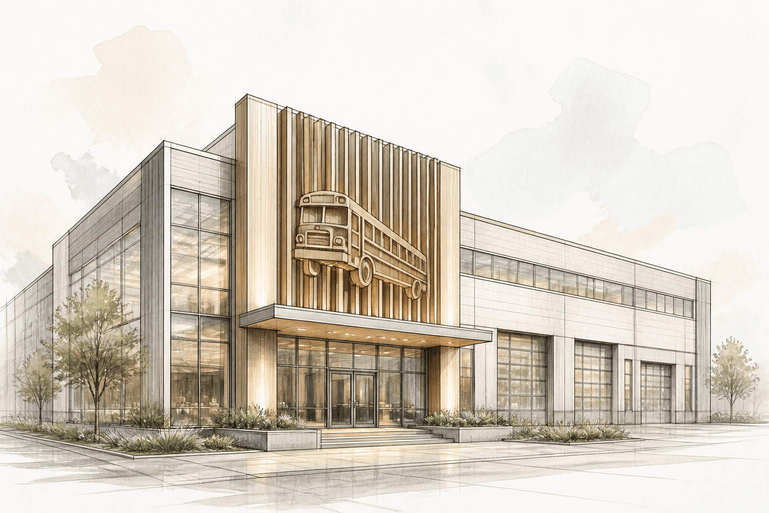
The model replicates a full-scale school bus production facility, from raw body frame fabrication and chassis integration to final paint, inspection, and delivery. It handles all three major bus classes — Type A (cutaway), Type C (conventional), and Type D (transit) — each with its own bill of materials, labor routing, and takt time on the assembly line. The financial core is built around operational physics: square footage of body, paint, and trim shops; shift patterns; and the interaction between chassis delivery schedules and body completion. This lets you test how a change in product mix, dual-shift adoption, or paint booth cycle time flows through to capacity, cost, and cash.

Revenue is structured around the industry’s typical multi-year fleet contracts alongside spot sales to districts and contractors. The model captures negotiated unit prices, option content (air conditioning, wheelchair lifts, camera systems), and staggered delivery dates that create uneven production loading and working capital swings. A dedicated input block for government procurement cycles and the school-year seasonality ensures that order intake patterns — and the resulting cash peaks — are modelled realistically, avoiding the trap of flat monthly revenue.

On the cost side, the build-up goes far beyond a simple margin percentage. A detailed BOM rolls up thousands of parts, from chassis (procured from external OEMs) to body panels, seats, lighting, and stop arms. Material cost drivers are linked to commodity indices where applicable. Direct labour is calculated station by station, with a learning curve during ramp-up and allowances for rework. The model also segregates energy-intensive paint shop costs, environmental compliance charges, and in-plant logistics, giving you a true gross margin per bus type. Warranty accruals are sized using historical claim rates and a tail-spend provision, so profit margins are not artificially inflated.

Modeling specifics

• Discrete production line model with body shop, paint shop, and final assembly stations, each with own capacity, buffer, and shift configuration; bottleneck analysis automatically identifies the rate-limiting step.
• Multi-class bill of materials (Type A/C/D) that distinguishes chassis cost, body-in-white, paint materials, and option content, with supplier price escalation curves.
• Fleet contract module with user-defined delivery schedules per contract, customized option take rates, and milestone payment terms that affect cash timing.
• Paint shop sub-model accounts for color batching, changeover time/materials, oven cure cycles, and VOC compliance cost per unit.
• Working capital simulation tied to chassis procurement lead times and seasonal order intake, exposing the real financing line needed before peak deliveries.
• Powertrain mix selector (diesel, propane, electric) that dynamically adjusts BOM, labour hours for high-voltage integration, and triggers infrastructure capex for EV charging.
• Learning curve applied to direct labour hours during production ramp-up, preventing gross margin overstatement in the first 6–12 months.
• Warranty accrual engine based on historical defects-per-bus and a compensation curve, plus a tail provision that prevents a profit spike after warranty expiry.

What's included in the base version

• Assumptions dashboard with macro drivers, sales volume, and product mix inputs
• Integrated production plan with takt time, shift schedule, and station-level labour
• Complete bill of materials with cost escalation and chassis procurement logic
• Revenue build-up from fleet contracts, spot sales, and option attach rates
• Direct & indirect operating cost structure (labour, energy, maintenance, logistics)
• Capital expenditure schedule with tooling, facility, and launch cost phasing
• Debt & equity financing waterfall with multiple tranches and DSCR covenants
• Monthly 3-statement model (P&L, Cash Flow, Balance Sheet) over 15–20 years
• Standard financial KPIs (IRR, NPV, payback) and sensitivity tables
• Executive dashboard with dynamic charts and one-click scenario selector

Common modeling mistakes

• Ignoring chassis delivery lead times and receiving chassis out of sync with bodies — production stalls eat 5–15% of annual capacity, making throughput and revenue projections unattainable.
• Modelling all bus types with identical assembly hours — labour cost per unit is distorted by 25–40%, hiding which products actually generate margin.
• Assuming immediate, linear ramp-up without a learning curve — direct labour cost in the first year is understated by 20–35%, inflating early EBITDA.
• Treating the paint shop as infinite capacity — bottleneck miss can overstate peak annual output by 20–30% and delay break-even by 6–12 months.
• Omitting seasonal order patterns and front-loading revenue evenly across months — cash balances appear 2–3x healthier than reality, masking the need for a working capital facility.
• Applying a constant warranty cost per bus without a tail provision — net profit is overstated by 1.5–3% of revenue from year 3 onward, and the balance sheet reserve is insufficient.
• Forgetting rollover of pre-delivery inspection and retrofits before bus sign-off — hidden labour and material costs cut 2–4% of unit margin.